Tables

• This is (mostly) from chapter 5.
  • You should read it.
• I am starting with the worksheet from the last set of notes.
  • Or you may start with yours.
• Start by making a copy of the Data worksheet
  • Call it Data as Table
  • Add it to the about sheet
• Tables in excel
  • This is a simple database like tool.
  • It facilitates sorting and filtering.
  • We will use these quite a bit.
• Building a table
  • As long as the data is contiguous
    • Select any cell in the table
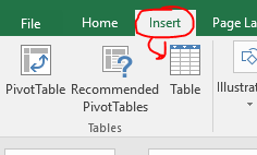
    • Insert->Tables -> Table
    • 
  • If it is not contiguous, make it so.
  • But you can also give a range
  • On the context dependent tab,
    • You can name/rename the table
    • 
• On page 111 he gives a list of benefits of a table.
  • We will want tables for pivot tables later.
  • They give us a quick way to explore the data.
• You can apply different styles to a table,
  • Or build your own, but I don't care about that type of task.
• Inserting into tables is somewhat easier.
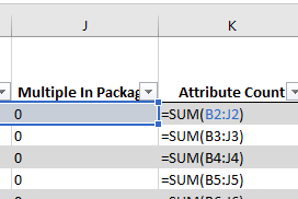
  • Go to column K, and insert a column to the left.
  • Call this column Attribute Count
  • in K2 put =sum(b2:j2)
  • Notice that excel copies this down for you.
  • 
• Play with filtering and sorting.
• Let's add a win rank column at the end.
  • I can never remember this function.
  • Let's use the formula editor
  • click in p2
  • Select the formula editor from the command bar
  • 
  • Search for rank
  • This gives us three reasonable choices.
    • Rank, which they tell us is for compatibility
    • rank.eq : the top rank is used for equally ranked values
    • rank.avg: the average rank is used for equally ranked values.
  • Select rank.eq
  • Notice the dialog box gives us information on the command
  • and there is a Help on this function in the lower left.
  • Select
    • Number: o2
    • Ref: win
    • Order : blank or 0
  • Reformat the column as integers.
• I would like to do something with the cost
  • Let's add a label column
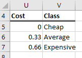
    • I want to break it into three categories, Cheap, Average, Expensive
    • Build a lookup table off to the side
    • 
    • Add a column after the price percentile column.
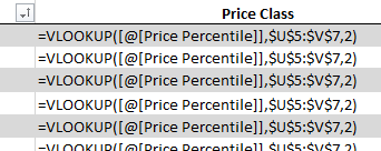
    • Do a vlookup on your new table.
      • =vlookup(
      • M2
      • $U$5:$V$7
      • 2
      • this is a range lookup, so the fourth parameter is not needed.
      • 
  • Can you do the same for Sugar Percentile but have four classes, low, Low, Low-Mid, Mid-High, High?
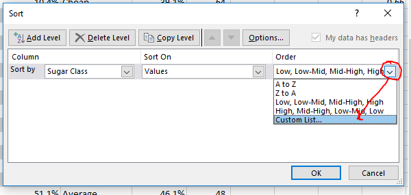
  • By the way, we can custom sort on these fields
    • Select the drop down menu in Price Class
    • 
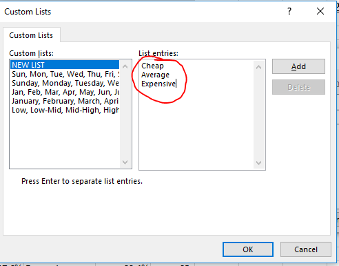
    • Under order, select the dropdown and select custom List
    • 
    • Type in the list under List entries
    • 
    • Now sort using this new list.
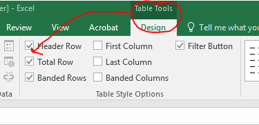
• A nice feature is the Total Row
  • Table Tools Design tab, Table Style Options, Total Row
  • 
  • Select Sum for columns b,c,d,e
  • Filter B for only values of 1
  • Filter D for only values of 1.
  • Notice the totals update to the filtered values.
• When filtering, excel hides rows
  • You don't want to work to the right of a table you are filtering.
    • Otherwise, your results will be hidden at times.
  • But you can copy and paste filtered data
    • And it will only copy the non-hidden rows.
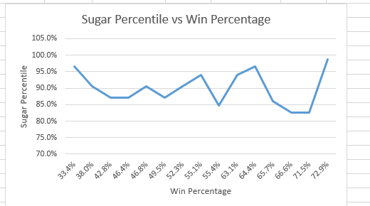
• If you produce a chart based on the data in the table,
  • As you filter and sort the data, the chart will change.
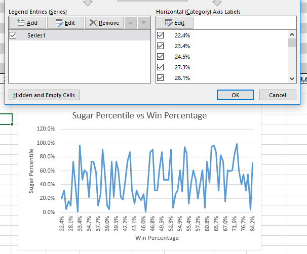
  • Build a line graph of Sugar Percentile.
  • Use Win percentage as the horizontal category
  • 
  • Put this below the table.
  • Filtering for only High sugar will change the graph
  • 
  • Move the graph to a new worksheet.
  • Create slicers.
• CandyC.xlsx