More Pivot Tables

• We will continue to use a cleaned version of the superheros dataset.
• This information is from page 492 in your text.
• Let's recreate where we were
  • Insert a pivot table.
  • Drag
    • Hair Color to Rows
    • Alignment to Columns
    • Name to Values
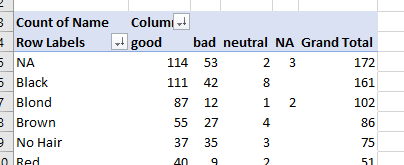
  • Sort the Columns descending by Count of Name.
• Sort the rows side by side by then number of heroes with black hair
  • Right click on a number in the black hair row
  • Select Sort -> More Options
  • 
  • Select
    • Largest to Smallest
    • Left to Right
    • 
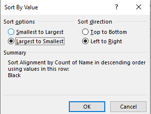
  • The result should move the columns around.
  • 
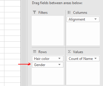
• I think I would like to look at gender as well.
  • Drag Gender into the Rows box, below Hair Color
  • 
  • Move it above Hair color
  • Drag it over to the Columns box
  • Move it around in this box
• This is nice, but I find that you can quickly build a chart that is very difficult to read.
• Let's start a new pivot table.
  • Make sure you use the cleaned data sheet to start.
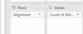
• Drag
  • Alignment to the rows column
  • Weight to the Values column
  • 
    • What did excel decide to do about weight?
• Since weight is a numeric field, we have more options.
  • On the Analyze tab in the Active Field command group
  • Note the currently selected column is named.
  • Click in the weight column if you have not done so.
  • 
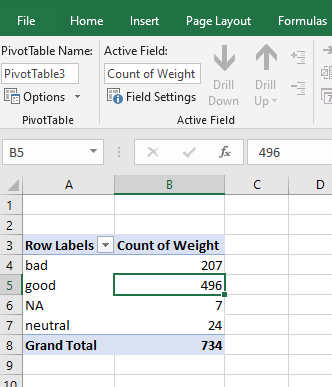
  • Active Field should contain Count of Weight
  • Click on Field Settings
  • 
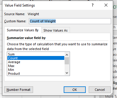
  • We have quite a few options here
    • Check out max and min
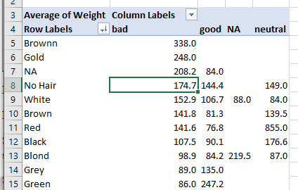
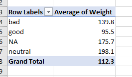
    • Try average
      • Looks like we should format that
      • But note there is a Number Format box
      • So format it to one decimal place.
    • 
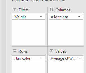
• Let's change it around a bit.
  • Move Alignments to Columns
  • Add Hair Color to Rows.
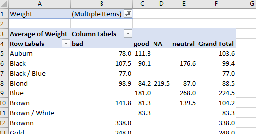
  • Why are some cells blank and some an error?
    • I bet it is the NAs
    • Let's add Weight to the filter area
    • And filter out the NAs
    • 
    • 
  • The Totals really don't make any sense any
    • Go to the Design tab in the Layout command group.
    • Notice you can use the Grand Totals to turn these totals on and off.
      • Let's add gender to the rows
        • Notice the Subtotals now make sense
      • Remove the Gender field
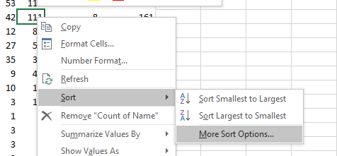
    • Sort the table based on the average weight of the bad characters
      • Right click on any bad weight.
      • Select sort ->more options
      • Select Largest to Smallest, Top to Bottom
      •