Vlookup
- The workbook for this set of notes is Hero2.
- There are several functions that allow you to look up a value in a table.
- We will discuss the Vlookup function today.
- Hlookup is very much the same, but for tables going the other way
- index/match is a more advanced combination for DSCI 201
- xlookup is a feature that is coming soon.
- Vlookup comes in two modes
- Exact match, look for a given value in a table.
- Range match, look for a value in a range.
- For all versions of vlookup we need a table.
- Arranged in rows of fields.
- The first field is the think we are trying to match
- The table we built last time is such a a table.
- We will start with exact lookup.
- For this we will try to find the height and weight for a given size category.
- We need the Size category to be the first column in a table.
- Setup
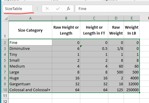
- First name the table to be SizeTable
- Highlight A2:E10
- Put SizeTable in the Name Box
-

- Then build a place to work
- In cell A22:C22 put the following
-

- Put Medium in cell A23
- The Vlookups
- In the exact form, there are no qualifications on the table.
- But the thing we are searching for must Match.
- We are trying to Find Medium in the table.
- We want to know the weight (from column 5) and the height (from column 3)
- Note that the columns are numbered from the start of the table, not from the start of the worksheet.
- The Index column is always column 1
- Vlookup takes the following parameters
- The thing you are looking for.
- In this case, it is the value in A23
- The table in which you are looking for the item
- In this case it is the SizeTable.
- The column number of the thing you want back
- we are looking for weight, so we want column 5.
- In the case of an exact match, the word False
- The actual lookup
- In cell B23 enter the following
- =vlookup(A23, SizeTable, 5, False)
-

-

- Change the value in cell A22 to something else and observe.
- Repeat this exercise, but this time look up the height for a given name.
- A ranged lookup allows us to find a value within a range.
- The table needs to have a range column as the first column.
- This needs to be arranged in ascending order. Smallest to largest.
- The lowest possible value needs to be the first value.
- The lookup will proceed as follows
- If the value is greater than or equal to the first value, but less than the second value, it will match the first.
- If the value is greater than or equal to the second value, but less than the third value, it will match the second.
- UP to the last.
- If it is greater than or equal to the last value, it will return the last value.
- Setup
- We need to build a new table
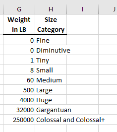
- Copy E1:E10 to column G, but paste as values
- Copy A1:A10 to column H
- Name E1:H10 as WeightTable
-

- We need a place to do the lookup
- In A25:B26 place
-

- The Lookup
- We are searching for a 20 in the Weight table, and we would like the second column back.
- Since this is a ranged lookup, we don't need the fourth parameters.
- =vlookup(a26, WeightTable,2)
-

-

- Why did it find Medium?
- Experiment with other weights.
- Repeat the exercise with a lookup for heights.
- Classifying the Weight
- We are missing one part, so I need to filter the data.
- Create a new worksheet, call it Cleaned Height and Weight.
- in A1:B2 put
-

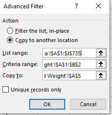
- Use this table and an advanced filter to get a new table with weights and heights not equal to na.
-

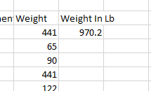
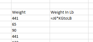
- Create a derived field, Weight In Lb
- Add a title Weight In Lb
- Under this add the formula =J6*KGtoLB
-

-

- Copy this down.
- Add a derived field Weight Category
- Add the title
- Enter the vlookup to lookup the weight in the Weight Table
-

-

- Copy this down.
- Repeat this process for Height.
