Tables

• Excel has a number of features that resemble a database.
  • These are tools that allow you to sort, filter and conduct sums on data.
  • While not a full database, these features are sometimes very helpful.
• For a table to work correctly the following should be true
  • The data should be arranged in records, which are stored in rows
    • 
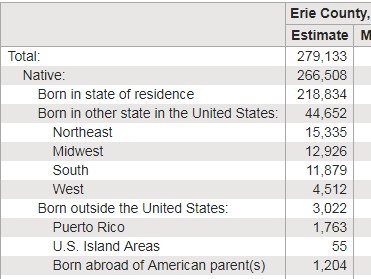
    • Not all rows are records, some are total rows.
    • To do anything, the totals need to be deleted.
  • The columns represent fields of the records
  • Only one data value per cell
    • 
    • This happens when there are not enough fields to hold the data.
    • Add another row.
  • All column data is of the same type.
    • 
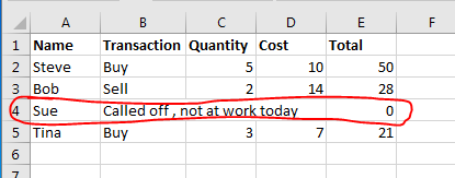
    • This frequently happens when someone is maintaining data by hand
    • They use a field to keep notes.
    • The extra data should be eliminated, or perhaps even the row.
  • The order of the rows is not important
    • 
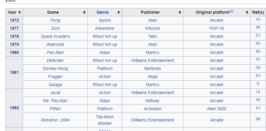
    • Note, the year needs to be duplicated across all records.
    • Sorting this data would cause many fields to lose the year
    • The entire row needs to be duplicated.
• It is also important, but not required, that each column has a heading.
• This is discussed on page 417/418 of the book.
• It is also part of This discussion
• Let's experiment with some of the table tools.
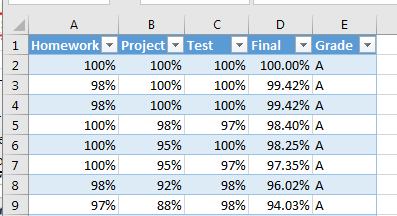
  • Start by making a new worksheet, Table and copy the data from the Cleaned Data sheet to this new sheet.
    • Notice, this satisfies all of the above conditions
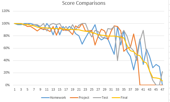
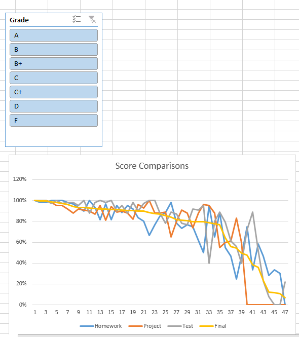
  • Let's quickly build a line chart showing all of the grades
    • Select all of the data.
    • Insert a line graph
    • Fix the title
    • 
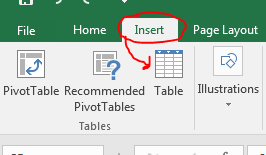
  • Click in any cell in the data.
  • On the Insert tab in the Tables workgroup, select Table
    • 
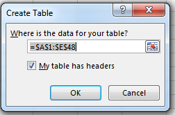
    • This will bring up the Create Table dialog
    • 
    • You can select a new range,
      • But if your data has no blank rows and no blank columns, then the correct value will be selected.
    • Also, check My table has headers
    • Then click ok.
    • 
  • On the new Table Tools, Design tab, select Insert Slicer from the Tools workgroup
    • 
    • This will bring up the Insert Slicers dialog
    • Select Grade
      • Since the slicer will want to display all of the data values, this is only really useful for the grades.
      • Or, in general, a field with a small set of values.
    • Clicking on OK will install a grade slicer.
    • Position this above the graph (so you can see both)
    • 
    • Explore
      • The check list box will change the way grades are selected
      • The filter will clear all selected items.
      • It is annoying that the graph readjusts, so move the graph and the slicer to another worksheet.
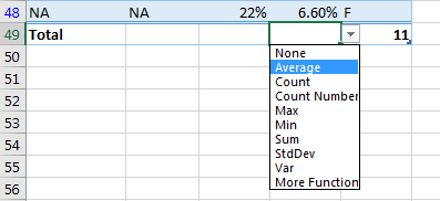
  • On the design tab, click on total row
    • 
    • This will add a new row at the bottom of the table
    • 
    • In this picture, I have only "F" selected in the slicer.
    • The number is a count of the values selected.
    • Let's calculate the average of the items selected.
    • Click in the final cell in the total row
    • Select average from the drop down menu.
    • 
  • Note: That using a slicer, or other filter function hides rows.
    • Copy and paste into areas with hidden rows causes problems.
    • Copy a table and paste it
      • Where data is hidden
      • Where data is not hidden.
  • Note that there are drop down menus for each of the columns
    • These can be used to sort and filter data in the column.
  • The Number Filter field needs some attention
    • Mixing filters is ok, but be careful you get what you want.
    • I tend to filter on one thing until I am comfortable
    • Notice that there are a number of pre-made filters.
    • Let's look at the project scores that are less than .7 but not equal to 0