The Height Column

• I want to begin by illustrating the different versions of count
  • I am going to work in cells M10 on, but you can work anywhere.
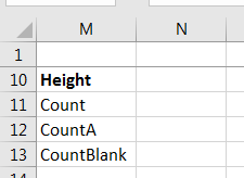
  • In M10, put Height, M11, Count, M12, CountA, M13 CountBlank
  • 
  • All three count functions we are going to investigate take a range.
    • A range can be in the form (Sm:En),
      • where S and E are letters, m and n are integers.
      • G1:G735 is the range we will use,
      • But G1:I22 is a valid range as well.
    • A range can also be (J:K)
      • This would include all cells in columns J and K
      • This is not good for what we will be doing.
    • A range can also be a (A1, B3, C4)
      • Just a list of cells.
    • And also a combination of the above.
    • Again we will use G1:G735
  • =count(range) will count any cell that contains a number.
  • =counta(range) will count any cell with data in the range, both numbers and letters
  • =countblank(range) will count any empty cell. Be careful, " " is not an empty cell.
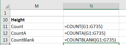
  • In cells N11:N13 put the following:
  • 
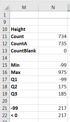
  • Notice the differences
    • Why are the values different?
    • What would =countblank(G:G) do?
• The five number summary consist of
  • Minimum data value
  • Maximum data value
  • Q1, Q2, Q3
• Max and Min
  • There are max and min functions.
  • They take a range and return the value.
    • Ignoring empty cells
    • Ignoring text cells
  • Put =min(g:g) and =max(g:g) in n15:n16
  • 
• Quartiels
  • Are measurements of position.
  • They divide the dataset into four sections.
    • The lower 25% of the values of the dataset are below Q1
    • Q2 is also known is the median
    • The lower 50% of the values of the dataset are below Q2
    • The lower 75% of the values of the dataset are below Q3.
  • Quartiles can be computed with three functions
    • =quartile(range, q)
    • =quartile.inc(range, q)
    • =quartile.exc(range, q)
    • In all three, range is the range of data to look at. (G:G) in our case
    • q is the quartile you want (1,2,3)
    • quartile is deprecated
      • 
    • The other two really don't matter. I will use quartile.inc
    • Put the quartile computations in n17:n19
    • 
  • You can do the same type of computation with percentile.
• Looks like we have a problem with -99
  • Let's explore countif just a bit more.
  • Remeber, this counts the values in a range that match a criteria.
  • Put -99 in cell m21
  • Put the formula =countif(g:g, m21) in cell n21
  • What does this do?
  • =countif(G:G, -99)
  • 
  • What does this do?
  • If we want, we can "ask" a more complex question with countif
    • Countif takes a range and a conditional test.
    • We can put cell values as we have done before.
    • We can also directly enter values
    • =countif(G:G, -99) will work just fine.
    • We can also put conditionals, but they must be in quotes
    • =countif(G:G, "< 0")
    • This will look for values less than 0.
    • 
• So far I have
• 
• Replace the -99 with a blank in column G
  • You know how to do this but...
  • Home Tab Find/Replace
  • Just let the replace box empty
  • Look at what that did to the count/counta/...
  • The numbers look just a bit better.
• Box and Whisker Chart.
  • This displays the five number summary
  • And identifies "outliers"
    • This is data that statisticians would say is probably "outside" of the norm.
  • Select column g
  • Insert tab, Charts workgroup, Insert Statistics Chart.
  • 
  • Select Box and Whisker chart.
  • I selected Layout 2 of the quick layouts.
  • And zoomed in a bit.
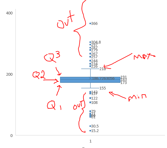
  • The Chart shows us
    • 
    • Q1, Q2 and Q3
    • The min and max of non-outlier data.
    • Outliers
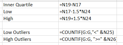
  • Non outlier data is determined by
    • low value is Q1- 1.5*(Q3-Q1)
    • high value is Q1- 1.5*(Q3-Q1)
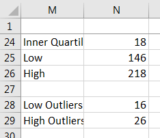
  • We can do a countif based on a conditional and a cell value.
  • It is a bit complex, but
  • =countif(range, "<" & cellref)
  • 
  • 
• I am fairly certain that we have a data problem with height
• This is a quick look at sorting, but it will help us with the data
  • Click somewhere inside of the main data area
  • Since the data is contiguous, the tool will select the entire table.
    • If we had a blank row or blank column we would have a problem.
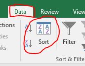
  • Go to the Data tab and select sort
  • 
  • Select Height and sort
  • 
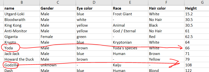
  • Look at the data, do you see a problem?
  • 
  • What should we do about this discovery?
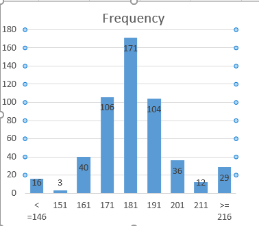
• A frequency distribution might be nice
  • We need to build bins so
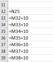
    • Enter =N25 in cell m32
    • Enter =M32+10 in M33
    • Drag this down to M39
    • 
  • We need a set of labels so
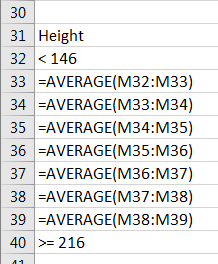
    • Enter &= 146 in cell N32
    • Enter =average(m32:m33) in cell N33
    • Drag this formula down to M39
    • Enter >= 216 in cell M40
    • 
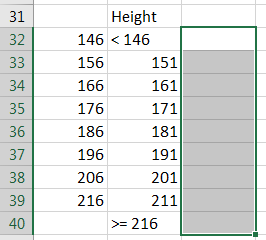
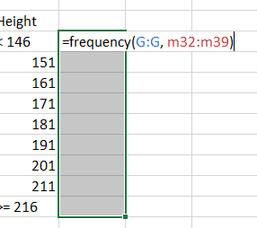
  • Now use the frequency function to compute the frequencies for each bin.
    • Select cells O32:O40
    • 
    • enter =frequency(G:G,M32:M39) and press ctrl-shift-enter
    • 
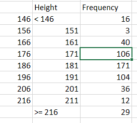
    • This will compute the frequency distribution
    • 
    • Values less than or equal to 146 are counted in cell O32,
    • Values between 147 and 156 are in cell O33
    • Values greater than or equal to 216 are counted in cell O40
  • Finally, draw a histogram with a clustered column chart.
  •