Computing Your Grade

• I would like to build a worksheet to compute your grade for this class.
  • This will be based upon our syllabus.
    • I tend to use percent based grade specification.
    • This means we will be doing weighted percentages
  • Other people use point based systems.
  • In any case, this is a good exercise.
• We will work in three phases
  • Build a worksheet to hold assumptions.
  • On a different worksheet, compute the percentages for each component.
  • Then compute the final grade.
• Worksheets are generally a good idea
  • You can break the computation down into more "workable" sections.
  • Making a computation fit on a single screen is helpful.
  • They do require some attention to detail however.
• Start excel.
• First build a worksheet for assumptions
  • Remember, assumptions are portions of worksheets that could change, but probably wont.
  • They are the components and weights for the class.
  • Rename the current worksheet
    • In the lower right hand corner, right click on the tab labels Sheet 1
    • Select Rename
    • 
    • Change the name to "Assumptions"
  • Create a worksheet for computations
    • Just click on the + sign in the lower left corner.
    • 
    • Rename this sheet to be "Computations
    • 
  • Worksheet controls
    • I tend to use lots of woksheets
    • This is my gradebook
      • four attendance sheets.
      • three grade sheets
      • 
    • Add a few more worksheets
    • The ellipsis on either side show that there are more worksheets
      • 
      • They can also be used for navigation
    • The arrows on the far left can be used to navigate as well
      • 
    • And the three horizontal dots can be used to resize the worksheet tab area.
      • 
  • Adding assumption data.
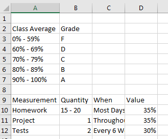
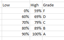
    • The assumptions for grades in this class are here
      • Open this in a tab on your browser.
    • You can copy and paste each of the tables into excel
      • Make sure you only get table data, or the paste will be difficult
      • 
    • An alternative method to copy and paste
      • Click anywhere on your worksheet.
      • On the Data tab, select Get External Data
      • Click on From Web
      • 
      • This may produce an error, but will also pop up a web browser.
      • 
      • Enter the url from above in the Address box and press Go
      • 
      • This should bring you to my web page
        • Scroll down until you see both tables.
        • Select the tables you want by clicking on the red arrow boxes.
        • Click on Import
        • 
        • This brings up an Import Data dialog box.
        • Select OK.
        • 
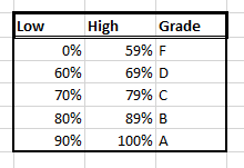
    • Formatting the First table.
      • Formatting a table will make it easier to read.
      • 
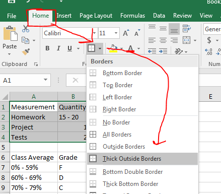
      • Highlight this table.
      • On the Home tab in the Font workgroup select the Borders menu
      • 
      • Select "Thick Outside Borders"
      • Highlight the column labels
      • Make them bold
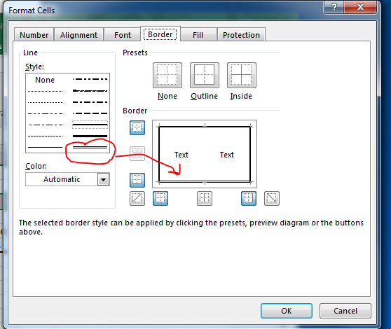
      • Drop down the borders menu again and select More Borders (at the bottom)
      • This will bring up the Format Cells dialog, with the Border tab selected.
      • Click on a single line style
      • Then click on the bottom border
      • 
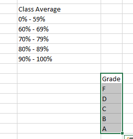
    • In order to use the Grade table, we need to modify it.
      • 
      • Highlight the grade column and move it out of the way.
      • The next command needs space to the right of the column.
      • 
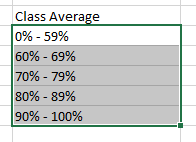
      • Highlight the percent ranges only
      • 
      • On the Data tab, in the Data Tools workgroup select Text to Columns
      • 
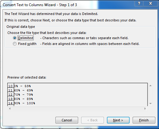
      • This will bring up the Convert Text to Columns wizard
      • 
      • We want Delimited, as our data is separated with a -, so click on next.
      • On the next step, select
        • space
        • other, and put - in the box.
        • Also select Treat consecutive delimiters as one
        • 
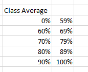
        • Selecting Finish will convert this data into two columns.
        • 
      • Change the labels and move the grades back.
      • 
    • You might find this technique useful in the future when dealing with your data set
      • You need space to the right of what you are splitting to hold ALL of the possible data.
      • We will revisit this in the future.
    • Format the grade table.
    • 
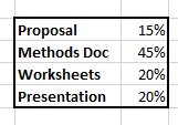
    • Add a table for the project
      • It is not a table in the syllabus so build it by hand.
      • 
• Computations
  • Move to the computations worksheet.
  • Homework
    • There are multiple homework assignments
    • Each could have different point values.
    • Let's build a simple table of this.
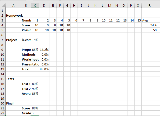
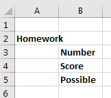
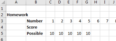
      • In the end, we want something like this
      • 
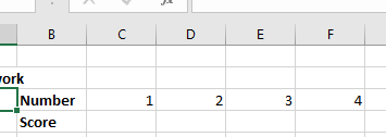
      • Top row, homework label.
      • Second row, points scored
      • Third row, points available.
      • Set up something like this
      • 
      • There might be 15 homework assignments, so fill c3:q3 with 1 2 3 ... 15
      • 
      • Highlight C:Q and shrink the column size
      • 
      • In R3 put the word "Avg"
      • We have had five homework assignments each worth 10 points. Fill in 10 in cells C5:G5
      • 
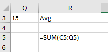
      • In cell R5, compute the total number of homework points
        • Use a sum function
        • Add all cells C5:Q5
        • 
        • 
      • Fill in grades for the first five homework assignments
        • For now use 10, 9, 8, 10, 10
        • Later use your grades.
        • 
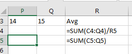
      • Compute the homework percentage
        • In cell R4
        • Sum the homework and divide by the possible sum
        • Mark this as a percent.
        • 
        • 
      • Try adding another homework score, don't forget to add the possible points.
  • Project
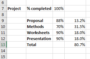
    • We want to build Something like this
    • 
    • Add the labels and the scores
    • 
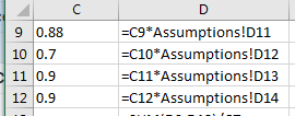
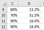
    • Now compute the weighted score for each part
      • This is the score times the weight.
      • The score is the value entered (88% for Proposal)
      • The weight is from the assumptions table.
        • Mine is C11:D14
        • If yours is not there, move it there.
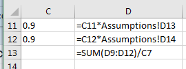
      • The computation is score*weight
      • 
      • 
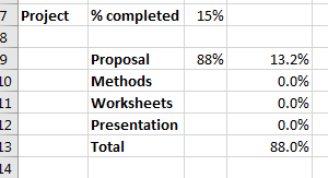
    • Finally, the total is the sum of the weighted score divided by the percent complete.
      • 
      • 
    • As portions of the project are complete, this will update the grade
      • Change all scores EXCEPT Proposal to blanks.
      • Change the %Completed to 15%
      • 
  • Tests
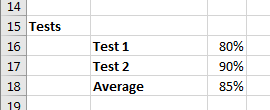
    • Add a title line and two lines to hold test scores.
    • Add a average line
    • Use some fake data for the tests
    • Later put your test score in and a 0.
    • Average the two tests
    • 
    • 
  • Final Computations
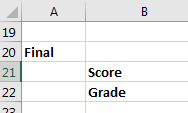
    • Add the following labels
    • 
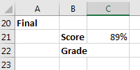
    • Calculate a weighted average of all course components
      • The homework percent is in cell R4
      • The project percent is in cell D13
      • The average of the test scores is in cell C18
      • The table of weights is in F4:F6 on the assumptions sheet.
      • Multiply each score by the weight.
      • 
      • 
    • Find the grade
      • We will use a vlookup to do this.
      • More on vlookup later but enter the following
      • 
      • 
  • The final worksheet
  •