Simple Finance Exercise

• Change the size of columns in an Excel workbook.
• Enter and format labels in cells.
• Enter and format data in cells.
• Enter and format simple formulas in cells.
• Enter and format simple functions in cells.

We will build on the idea of a check register from last time, but we will allow for a number of different categories of expenses, Housing, Food, Clothes, Transportation, Entertainment and Miscellaneous.

1. Start excel.
2. Enter the column headings as pictured
   • 
3. Adjust and format the column headings.
   • Make the Description column approximately 30 pixels wide.
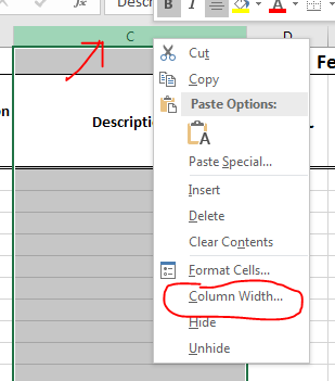
     • Click on the heading of the column (C)
     • Right click and select "Column Width"
     • Set the width.
     • 
   • Use the wrap text button in the alignment workgroup of the home table to allow "Transaction Number" to take up two lines.
   • Use the orientation button in the same workgroup to rotate each of the categories.
   • Change row 2 so that everything fits.
   • Center Date, Transaction Number and Description horizontally and vertically (Alignment group again.)
   • Make all columns past the description 10 points wide
     • Select columns d-k
     • Repeat the first step.
   • 
4. Enter the following transactions

   • Date	Transaction No	Description	Category	Amount
     2/1		January Balance	Balance	1000
     2/1	10000	Pay	Deposit	750
     2/1	10001	Rent	Housing	450
     2/3	10002	Giant Eagle	Food	145.67
     2/3	10003	Armstrong Cable	Entertainment	87.33
     2/3	10004	Compadres	Food	25.19
     2/5	10005	Walmart	Clothes	55.92
     2/5	10006	GetGo	Transportation	42.87

   • Format all of the number fields correctly, including the Balance column.
5. Compute the balance column
   • For K4, start with K3, add D4 and subtract the values in E4 through J4.
   • But I would subtract the sum of E4 through J4, not have a bunch of minus terms.
   • Copy this down K5 through K10.
   • 
6. Add a total line
   • Draw a double border under row 10
   • Add "Totals" to D11, make this bold and right aligned.
   • In E11 through J11 total each column.
   • Add a double check in K11
   • 
7. Add Another worksheet
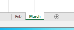
   • At the bottom of the page click on the + button
   • 
   • This will add another worksheet
   • Right click on the worksheet and rename it, "March"
   • Rename the first worksheet "Feb"
   • 
8. Copy A1:K2 from the Feb worksheet to the March worksheet.
   • Selecting Paste will make this easiest.
   • You will still need to reset column widths.
   • Change the top cell to be March.
9. Link the Feb balance to the March worksheet
   • Click in cell K3 on the March worksheet.
   • enter =
   • Click in cell K10 on the Feb worksheet.
   • Press enter.
   • The following formula should show up in the March workbook
   • 
10. Enter the following transactions

    • Date	Transaction No	Description	Category	Amount
      3/1		February Balance	Balance
      3/1	10007	Pay	Deposit	750
      3/1	10008	Rent	Housing	450
      3/3	10009	Armstrong Cable	Entertainment	87.33

11. Make up at least three more transactions for this month and record them.
12. Calculate the balance as in instruction 5.
13. Calculate the totals as in instruction 6.
14. Save your work
15. Submit your saved document to the Simple Accounting folder in the Assignment section of D2L for this class.