Cereal Stats

• Imported a CSV file.
• Used various statistical functions.
• Sorted data.

1. Download this file. Save it somewhere you can find it.
   • This is a comma separated value file.
     • Data is in rows, with commas between the values.
     • Excel will be happy to load this file, just make sure to tell it the fields are delimited with a comma (,) not spaces.
     • Once the file is opened, save it as an excel file.
       • File
       • save as
       • Select excel workbook.
2. Information step: the data in this file consists of:
   • The name of the cereal:
   • The manufacturer:
     • A = American Home Food Products
     • G = General Mills
     • K = Kelloggs
     • N = Nabisco
     • P = Post
     • Q = Quaker Oats
     • R = Ralston Purina
   • type:
     • H = hot
     • C = cold
   • calories: calories per serving
   • protein: grams of protein
   • fat: grams of fat
   • sodium: milligrams of sodium
   • fiber: grams of dietary fiber
   • carbo: grams of complex carbohydrates
   • sugars: grams of sugars
   • potass: milligrams of potassium
   • vitamins: vitamins and minerals - 0, 25, or 100, indicating the typical percentage of FDA recommended
   • shelf: display shelf (1, 2, or 3, counting from the floor)
   • weight: weight in ounces of one serving
   • cups: number of cups in one serving
   • rating: a rating of the cereals (Possibly from Consumer Reports?)
3. Adjust the columns so everything fits on the screen.
   • 
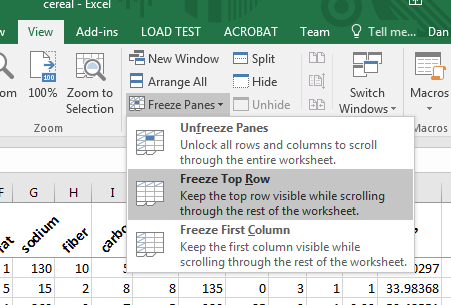
4. In large worksheets like this it is nice to freeze the headings
   • On the View tab.
   • In the Window workgroup
   • Select the Freeze Panes drop down
   • Select Freeze Top Row
   • 
   • This will keep the top row visible as you scroll down in the data.
5. Sort the data.
   • I want to see the most popular types of serial in both hot and cold.
   • Sort with a first level on type and the second level on rating.
   • Make sure that the hot cereals are first and the highest rated is at the top.
   • 
6. Clean the data
   • There are several fields containing a -1. I doubt that this is good data
   • Use find and replace to find all occurrences of -1 and replace them with a space.
   • I had 4 values replaced.
7. Do some basic statistics
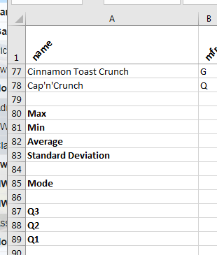
   • Move to the bottom of the data and insert the following labels
   • 
   • Using the appropriate function, calculate the statistics for all columns D through P
   • I used max, min, average, stdev.p, mode.sngl, quartile.inc
   • 
   • It probably doesn't make sense to compute the statistics on the "shelf" column, so remove these for column M, (clear contents)
   • Note, there is no mode for the rating.
8. Count the types by brand
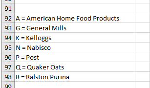
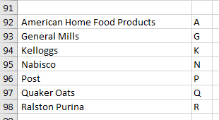
   • Copy the list of manufactures from above and paste it into a92:a98
   • 
   • Split this data into two columns
     • Highlight the range
     • Data tab, Data Tools workgroup, Text To columns
     • The data is delimited by an =
   • 
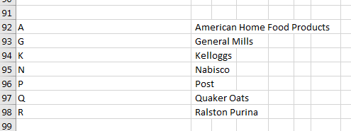
   • Rearrange the columns so the manufacturer name is in column A and the letter is in column B.
   • Each of the letters in B92:B98 has a space at the end.
     • These need to be removed.
     • There are several ways to do it, but just deleting the spaces in the 7 cells is probably the easiest at this point.
   • 
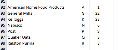
   • Use the countif function to compute the number of cereal types from each company
     • In cell c92, enter =countif (or use the insert function button)
     • The first argument is b2:b78
       • The the list of manufacturers.
       • We want to count the number of times each letter occurs.
       • We will copy this formula down, so use an appropriate mixed reference
     • the second argument is b92
       • This is the thing we want to count.
       • We want this cell reference to change as we move down.
       • If you did not delete the spaces the result will be 0, otherwise it will match the values pictured.
     • 
   • Label this computation
9. Build a table to count the number of hot and cold cereals.
   • I know you can just count them, but practice the procedure.
   • Do this in cells a100:c102
   • 
10. Save your work
11. Submit your saved document to the Cereal folder in the Assignment section of D2L for this class.