Chapter 2 of Excel

• I have somewhat of a schedule conflict on Thursday so
  • I will be here for part of the day on Thursday and Dr. Meyer will be here for the rest.
  • I will talk on both days.
• This section covers two things.
  • Absolute vs relative vs mixed addressing.
    • This is not hard, but rather a new skill most people need to learn
  • Functions.
    • This is both easy and hard.
    • It is easy as the functions do the work for you.
    • It is hard in that you need to learn the functions and when to use them.
    • This is the page numbering thing all over, pay attention.
    • Oh, and I would keep a list of functions, what they do and how to use them.
• Let's do a loan.
  • Loans are the way we purchase many large items.
    • Think car, boat, house, education, ...
    • The loans we are talking about here are installment loans
    • For a fixed period.
  • Most loans require three pieces of input
    • The amount borrowed.
    • The period of the loan
    • The interest rate of the loan.
  • Sometimes we need to compute the down payment and amount financed.
• Let's say we want to purchase a house for $150,000. We plan to pay for 30 years at an interest rate of 4.3%. The bank requires a 20% down payment.
• We want to do several things.
  • Compute the monthly payment.
  • Compute the amount of interest paid
  • Compute the amortization table.
• Start by placing "cost of house" in a1 and $150,000 in B1
• Put Percent Down in A2 and 20% in B2
• Put Down Payment in A3
• Calculate the down payment in cell B3 (=b1*b2)
• Put Amount Financed in A4
• Calculate the amount financed in B4, (=b1-b3)
• Put "Term" in cell A5 and 30 in cell B5
• Put "APR" in cell A6 and 4.3% in cell B6.
• Put Payment in cell A7
• We are going to learn to use the payment function
  • m = P(r/n)/(1-(1+r/n)^(-nt)) is the formula.
  • But you will get this wrong.
  • So excel has a payment function.
  • It takes three parameters
    • The monthly interest rate
    • The number of payments
    • The amount financed.
  • We have a version of all three of these.
    • The monthly interest rate is the APR (4.3%)/12
    • The number of months is the term (30)*12
    • The Amount financed is the -Amount financed.
  • So in cell B7 put =pmt(b6/12, b5*12, -b4)
  • End of discussion. Learn to do this, don't argue.
  • Ok, two discussion points
    1. Sometimes you don't make monthly payments.
       • In that case, don't divide and multiply by 12, but by the payments per year.
    2. Make sure that the term is given in years, not months, otherwise you don't need to multiply by 12.
    3. Let's calculate the total amount paid and the total interest paid.
       • In cell A9 put Total Paid
       • In cell B9 compute the total of all payments, don't forget to include the down payment. (=b7*b5*12+b3)
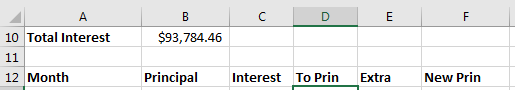
       • In cell A10 put Total Interest
       • In cell B10 compute the total interest (=b9-b1)
    4. 
    5. We will now build an amortization table
       • This shows you how the loan stands for each month.
       • Across row 12 put the following
         • Month
         • Principal
         • Interest
         • To Prin
         • Extra
         • New Prin
       • 
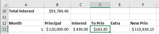
       • In column A, we want to place the month.
         • Just put 1 in A13, 2 in A14, 3 in A15
         • Highlight these three and drag down to A372.
       • In column B we want to calculate the current amount due.
         • This will be a two stage process. First just copy the amount from cell B4 (=b4) into B13
         • We will do the next step later.
       • In cell C13 we want to compute the interest due this month.
         • This is a simple interest computation (i=prt)
         • The principal is in cell b13.
         • The interest rate is in cell B6, but this needs divided by 12
         • The time is 1 month.
         • So put the formula (=b13*b6/12) in cell c13
         • We will modify this later.
       • In Cell D13 we want to compute the part of the payment that goes toward principal.
         • This is just the monthly payment (b7) minus the interest due this month (c13)
         • In Cell D13 put (=b7-c13)
         • We will change this later.
       • E13 should be blank for now.
       • In F13 we wish to compute the principal after the payment is made
         • This is just the starting principal minus the amount to principal and any extra payment
         • Enter (=B13-D13-E13) in cell F13
       • 
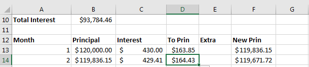
       • We are now ready to compute row 14
         • Where should the value for B14 come from (=F13)
         • Can we copy the other formulas down?
           • If I do, I owe $5,930,349.04 in interest, this does not seem right.
           • Look at the formula
             • =b14*b7/12
             • This is using the monthly payment as the interest rate
             • Why?
             • Remember last time when we copied formulas in the checking book.
               • If we copy a formula down the numbers go up.
             • That is sort of what we want to happen here.
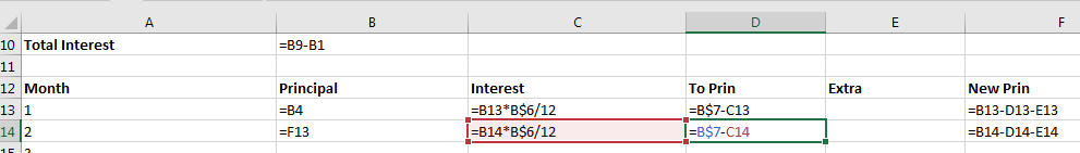
               • We want the number associated with the principal to change from B13 to b14
               • But we don't want the interest rate cell to change
             • To keep this from happening, we can put a $ in front of the thing we don't want to change
               • In this case, we don't want the 6 to change
               • So the formula in cell C13 becomes (=b13*b$6/12)
               • Copy that down and see what happens
               • It works!
           • So what modifications to we need to make to the formulas in cells D13 and F13? and WHY?
             • D13 should become (=b$7-c13)
             • F13 does not need to change.
           • Copy these formulas down to row 14.
           • 
           • 
       • We can now finish this table.
         • Highlight cells b14:f14
         • Double click in the box in the corner.
    6. The use of the $ in a formula changes the mode of addressing
       • no $ is relative cell reference =b4-c2
       • a $ in front of everything is a absolute cell reference =$b$3*$c$5
       • Some $ and not some $ are called mixed references =b$3/$c5
    7. What happens when each of these is in cell d5 and copied to cell e6
       = a1 = $a1 = a$1 = $a$1
    8. When do you put a $ in a cell reference
    9. By the way, F4 (the key) circles through the various options.