Final Exam, CSCI 104 Summer 2012

Instructions

The final product should be neat and organized. Extraneous data, computations or annotations will result in a loss of points.
Whenever possible, you should demonstrate your ability to use excel as a tool. Compute values whenever instructed to do so. Values entered by hand which should be calculated will result in no credit for that portion of the test.
It is your responsibility to save and submit your document properly, this is part of the test. If I do not receive a copy of your final document, you will receive zero credit for this portion of the test.
If you have a question about the instructions, please ask. If you have a question about excel, you may ask but please don't expect an answer.
Screen shots of individual portions will be spread throughout the document.

Startup
1. Download this file to your student work area.
2. [1 point] Save it as Excel_Final_Lastname_Firstname.xlsx
3. This document contains several worksheets
  - Canyon Data is related to the base price of a 2012 GMC Canyon.
  - Movie Data is related to the top 100 grossing movies of all time.
  - Island is related to purchasing an island paradise.
Canyon Configuration Sheet
1. Switch to the Canyon Data Worksheet
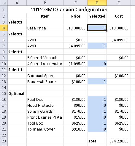
2. The goal is to create a worksheet where you can configure a Canyon to your specifications.
3. [1 point] Merge cells A1:E1 and insert the title 2012 GMC Canyon Configuration
4. [1 point] Format the title as bold, 14 point and centered.
5. [1 point] Format the cells containing Select 1 and Optional as bold.
6. [1 point] In cells B2 through E2 enter the following (centered and bold)
  - Item
  - Price
  - Selected
  - Cost
7. [1 point] Color Cells D4, D7, D10, D13, D16:21 light blue. These cells will contain either a 0 or a 1, used to select the options.
8. [1 point] Cell E4 should reference cell C4, since the base price must be selected.
9. [10 points] In cells E6, E9 and E12 compute the price for a required selection.
  - All computations are the same, so develop a formula which can be copied from E6 to E9 and E12 without change or editing the formula.
  - If the value in cell D7 is a 1, then the consumer has selected the 4WD option, and the price for this option (C7) should be displayed in cell E6, otherwise the price of 2WD (C6) should be displayed.
  - Copy this formula to the other cells without modification.
10. [4 points] In cells E16:E21, compute the price of the specified options.
  - Again, all of the formulas are the same, develop one and copy to the rest.
  - If the customer places a 1 in cell D16, then E16 should contain the price of the fuel door (C16), otherwise a 0.
11. [1 point] Use a formula to compute the total price of this truck in cell E23, and place the label Total in cell D23.
12. [1 point] Format all dollar amounts as currency, displaying the dollar sign next to the number, and 0 displays as $0.00, not -.

Loan Information

[1 point] Insert a new sheet, named Loan

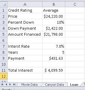
[2 points] In this new sheet, insert the following labels

Cell	Value
A1	Credit Rating
B1	Average
A2	Price
A3	Percent Down
A4	Down Payment
A5	Amount Financed
A7	Interest Rate
A8	Years
B8	5
A9	Payment
A11	Total Interest

[5 points] Insert the following table so that the credit rating in cell A1 can be used to find the Interest Rate and Down payment.
- This should be in cells F2:H6 (Be careful and get this right)
- You will need to adjust the table.
- Rating Interest Rate Down Payment
  
  Poor 8% 15%
  
  Average 7% 10%
  
  Good 5.8% 7%
  
  Exceptional 5.3% 0%
Link Cell B2 to the total (E23) on the Canyon Data page.
[4 points] Using the table in cells F2:H5 and the value in cell B1, compute the required percent down in cells B3.
[1 point] In cell B4, compute the down payment using the values in cells B2 and B3.
[1 point] In cell B5, compute the amount financed using the values in cells B2 and B4.
[4 pints] In cell B7, compute the interest rate based upon the credit rating in cell B1 and the table in cells F2:H5
[3 points] In cell B8, compute the monthly payment based upon the terms listed in the cells above.
[3 points] In cell B11, compute the total interest paid for this loan.
Make sure all fields are formatted correctly.
Change the credit rating in cell B1 to Good.

Island Purchase
1. Switch to the Island worksheet.
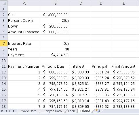
2. [5 points] Compute the monthly payment for a loan based upon the information supplied on this worksheet. (Cells B4-B9)
3. [10 points] Complete the Amortization table in cells A12:E371
4. [5 points] If all other terms remain the same, determine the price of the island which can be purchased with monthly payments of $2500. Keep the results of your findings in your worksheet.
Tables
1. [2 points] Make a copy of the Movie Data called Movie Table and move this after the Island worksheet.
2. Move to the Movie Table worksheet.
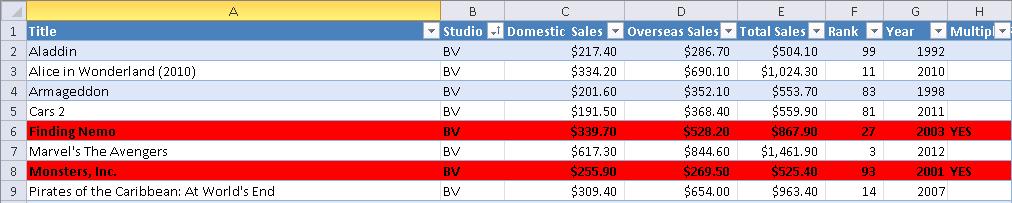
3. [1 point] Convert the data on this worksheet to a table.
4. [2 points] Sort the table by studio, then by title within each studio.
5. [2 points] Insert a new column to the left of Overseas Sales called Total Sales and contains the sum of Domestic Sales and Overseas Sales.
6. [3 points] Insert a total line at the bottom of the table which computes the sum of each of the following columns: Domestic Sales, Overseas Sales and Total Sales
7. [3 points] Insert a column to the left of Total Sales called Rank which computes the ranks of the movies based upon Total Sales
8. [4 points] Add conditional formatting so that moves which are in the top 20 , and were released multiple times (A YES in column H)
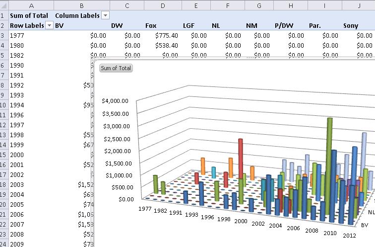
Pivot Tables
1. Create a new worksheet called Pivot
2. [12 points] Using the data in Movie Data Create a pivot table.
  - Use the Studio as the column label
  - Use the Year as a row label
  - Display a calculated field which displays the total sales (domestic + overseas)
3. [4 points] Insert a pivot chart to accompany this table.
  - Use a 3d Cylinder chart, style 2.
Email a copy of your file to danbennett360@gmail.com
Have a great day.

Rating	Interest Rate	Down Payment
Poor	8%	15%
Average	7%	10%
Good	5.8%	7%
Exceptional	5.3%	0%