Please turn in your written portion now.
You print a copy of this test if you wish, but that is not required.
If you get stuck on a section, move on to something else.
Point values are given by each instruction.
If you don't understand an instruction, ask for help.
Make sure you format all data correctly. Points will be deducted for poor formatting.
Make sure you save your worksheet often to permit disaster recovery if necessary.
When you are finished, you should email your workbook to dbennett@edinboro.edu. Failure to do this will result in loss of all points associated with this portion of the test.

Start excel.
Filtering and Sorting
1. (2 points) Import the text file chap5_cap_airlines into your worksheet.
  If you don't have your data, a copy is here
2. (1 point) Rename the tab Raw Data
3. (2 points) Convert this data to a table.
4. (1 points) Apply table style light 8 to this table.
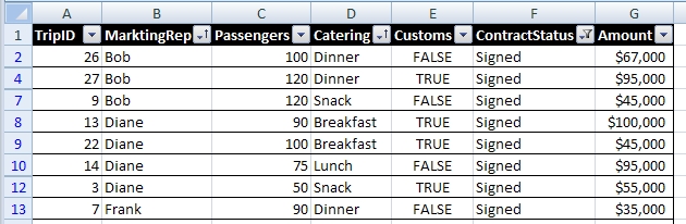
5. (1 points) Filter the data to show only Signedcontracts.
6. (1 point) Sort the data by Marketing Rep, then by Catering type.
7. Your data should look something like
Pivot Tables (12 points)
1. Create a pivot table.
2. Rename this tab Sales
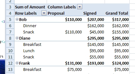
3. The body of the table should contain a report of the total sales Amount for each MarketingRep.
4. The columns should be by ContractStatus
5. There should be a sub Section for each Marketing Rep
6. The MarketingRep data should be broken down by Catering type.
7. The table should be appropriately formatted.
8. Your data should look something like
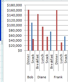
9. Create a clustered column chart summarizing this data.
10. Your chart should look something like

Mortgage Payment

(1 point) Make a new worksheet, name this Mortgage
(1 point) Place your name in cell B3.

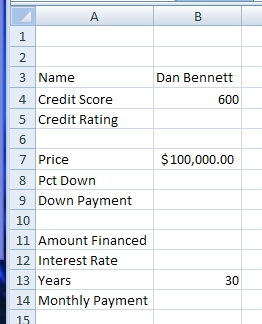
(5 points) Enter the following data.

Cell Reference	Cell Data
A3	Name
A4	Credit Score
A5	Credit Rating
A7	Price
A8	Pct. Down
A9	Down Payment
A11	Amount Financed
A12	Interest Rate
A13	Years
A14	Monthly Payment
B4	600
B7	100,000
B13	30

(3 points) Build the credit table pictured below.
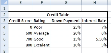
(2 points) Using a function, place the customer's credit rating in cell B5, based on the credit score in B4 and the Credit Table.
(2 points) Using a function, place the customer's required percentage down in cell B8, based on the credit score in B5 and the Credit table.
(1 point) Compute the down payment based on the price of the house and the customer's required down payment percentage. Place this value in B9
(1 point) Compute the amount financed in cell B11.
(2 points) Using a function, place the customer's interest rate in cell B12, based on the credit score in B5 and the Credit table.
(3 points) Compute the monthly interest payment for this loan in cell B14.

Mortgage Table
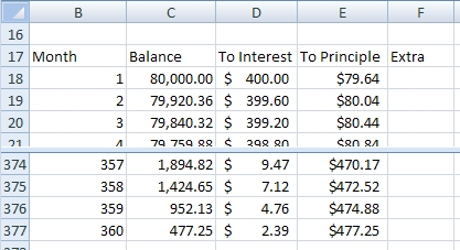
1. (2 points) Enter the following data.
  
  Cell Reference Cell Data
  
  B17 Month
  
  C17 Balance
  
  D17 To Interest
  
  E17 To Principle
  
  F17 Extra
2. (2 points) Put entries for 360 months in cells b18 to B377
3. (2 points) Split the screen so that B374 to B377 are visible as well as the top of the mortgage table.
4. (2 points) In cell C18, link to the Amount financed in cell B11.
5. (4 points) In cell D18, calculate the amount of interest due the first month. Make this a formula which can be copied to the remainder of the table.
6. (4 points) In cell E18, calculate the amount applied to the principle for the first month. Make this a formula which can be copied to the remainder of the table.
7. (4 points) In Cell C19, calculate the new Balance, this should be based on the previous balance, the amount to principle and the extra payment in cell F18. Make this formula so that it will never become zero.
8. (4 points) Complete the Mortgage table.
9. Final Instructions
  - (5 points) Find the average, max, min, and total interest paid. Place these values in cells H10:H13, with appropriate labels in G10:G13
  - Place 100 in cells F18 and F19
  - Place 750 in cell B4
  - Place 200,000 i cell B7
  Email your final worksheet to dbennett@edinboro.edu