Excel Test, Spring 2006

Please perform the following task.

• Make sure to save often so that if you lose your work, you can continue.
• When you are finished, print the resulting spreadsheet in formula mode.
• You may use your book.
• Use a different area of the spread sheet for each problem.
• Label all assumptions.
• Format all data values correctly.
• Red lines have been added to all pictures to discourage cheating.

Use Excel to answer the following Questions:

• Open this worksheet. You should probably save it to your S drive and open it from there.
• Part 1, 10 points.
  • Label the sheet "Part 1"
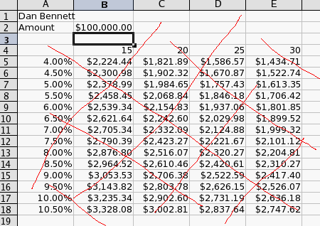
  • In A2 place the word Amount
  • In B2 place $100,000
  • In cells B4-E4 place the values 15, 20, 25, 30
  • In cells A5-A18 place the values 4%, 4.5%, 5%, ... 10%, 10.5%
  • In cell b5, develop a formula that calculates a payment for a loan for the amount in cell b2, for the interest rate as listed in column a5-a18, for the period of years listed in B4-E30. This should be for quarterly payments.
  • Copy this formula to cells b5-e18. There should be a single formula with proper cell references, I will be looking for this.
  • Change the amount to be $50,000 in cell b2.
  • Here is a picture of my sheet.
• Part 2, 15 points.
  • Move to the second sheet.
  • Label the sheet "Part 2".
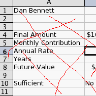
  • In cell A1, place your name.
  • In cell A4 Place "Final Amount"
  • In cell B4 place 100,000
  • In cell A5 place "Monthly Contribution"
  • In cell B5 place $100
  • In cell A6 place "Annual Rate"
  • In Cell B6 place 5%
  • In cell A7 place "Years"
  • In cell B7 place 30
  • In cell A8 place "Future Value"
  • In cell B8, compute the future value of this investment. Remember, the amount in B5 is a monthly contribution.
  • In cell A10 place "Sufficient"
  • In cell B10, use a formula or function to place the word "Yes", if the value in B8 exceeds the value in cell B4, and a "No" otherwise.
  • Change the value in cell b5 to be 130
  • Here is a screen shot of my work
• Part 3, 25 points.
  • Move to worksheet Part 3.
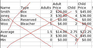
  • Using the lookup function, compute the price for the adult, child and senior tickets in the table A9-K13
  • Compute the discount based on the table in G2-H6 and the total price. This should involve a formula.
  • Compute the discount price based on the total price and the discount amount
  • Compute the total price for each row.
  • Format the table, including making all prices and text fit, coloring labels, and formatting values.
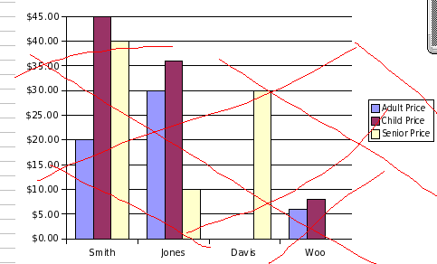
  • Create a column chart
    • showing the price by family
    • with the contribution of each type of ticket displayed as a different bar.
    • Make sure that the family names, as well as the ticket types are labeled.
    • 
  • Add, in row 15, an average line for columns C-I and K
  • Add, in row 16, a maximum line for columns C-I and K
  • Add, in row 17, a minimum line for columns C-I and K.
  • 
• When you are finished, Print each of the worksheets in formula view.
• Email a copy of the worksheet to dbennett@edinboro.edu. You will receive a 10 point penalty if you fail to perform either of these steps.