Excel Test, CSCI 104, Spring 2004
Please do the following exercise.
At the end of class, you must print this out in formula mode
and turn it in.
In this work, we will design a worksheet for selling prebuilt homes.
Boxes coloed blue will contin values you will change to reconfigure
news units.
You may use the numbers I provide to develop your worksheet, but in the
end you will be asked to put in a new set of values for the final project.
- Build a table of options for configuring the prebuilt homes.
- In Columns A-F, Rows 1-6 place the following information
| Base Package |
|
|
|
Features |
|
| Model Number |
Description |
Price |
|
Number |
Price |
| 123 |
Base Model |
$45,999 |
|
0 |
0 |
| 133 |
Standard Edition |
$55,999 |
|
100 |
$5,000 |
| 155 |
Deluxe Model |
$72,999 |
|
200 |
$9,000 |
| |
|
|
|
300 |
$12,000 |
- Build a configuration area.
- in cells a7-f7 place the words "Dan's Prebult Homes".
- Change the font to be 20 point, change the font to be some
form of script, center the title. (You may change the name
if you wish)
- In Cell A8 place the label "Customer Name"
- Color B8 blue, put your name there.
- Cell D8 should contain the label "Options"
- Cell A8 should contain the label "Model Number"
- Cell B9 should be colored blue, put the number 123 here.
- Cell D9 should contain the label "Number"
- Cell E9 should contain the label "Price"
- Cell A10 should contain the label "Model Name"
- Cell B10 - look up the name in tabel 1, cells A3-c5, this should be "Base Model" but should change when a new value is put into B9
- Cell D10, place the number 0, color the cell blue
- Cell E10, Lookup the price for the opton in D10 in table 2, E3:F6,
this should change if you change the number in D10
- Cell A11 place the label "Base Price"
- Cell B11, look up the price based on cell b9 and table 1
- Cell D11, E11 do the same as cells D10 and E10. Place 100 in D11
- Cell A13 should contain the label "Total"
- Cell B13 should be the sum of cells B11, E10, E11
- Financing Information
- Cells A15:F15 should contain the label "Financing Information", centered in 20 point font.
- Cell A16 should contain the label "Down Payment"
- Cell B16 should be blue. Place the number 5000 in this cell.
- Cell A17 should contain the label "Discount"
- Cell B17 should be blue, place the number 2000 in this cell.
- Cell A18 should contain the label "Tax"
- Cell B13 should contain the the final price with discount removed multiplied by 6%
- Cell A10 should contain the string "Amount Financed"
- Cell B20 should be the total price, minus the discount and down payment plus the tax.
- Financial functions
- Build a table in cells A22:E26,
- Place the following values: B22 15, C22 20, D22 25, Edd 30
- Place the following values: A23 7%, A24 8%, A25 9%, A30 10%
- Develop a single formula in cell b23
- Compute the monthly payments ont he amount financed, for 15 years at 7%
- This formula should be copied to all other cells in the table without changing it.
- This is a test of your ability to use the payment function as well as absolute vs relative addressing.
- Gratuitous Chart
- Using cells B23:E26 create a chart
- The title should be "Gratuitous Chart"
- The type should be a 3d line chart
- Label the Z axis "Amount Financed"
- Label the Y axis "Years Financed"
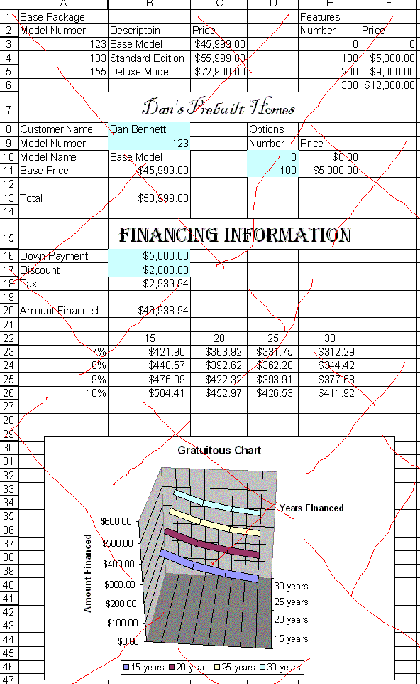
- Try to make the chart match mine as closely as you can.
- Put the sheet in formula mode
- Change the following values
| B8 | Your Name |
| B9 | 155 |
| D10 | 200 |
| D11 | 300 |
| B16 | 10,000 |
- Make sure your name is on the work.
- Make sure that your sheet is in formula view (I will deduct 20% if it is not)
- Your sheet should be printed with grid lines on.
- You will probably have 3 pages, collect them all.
- Print it out and turn it in.
- My work
- Here are pictures of my prototype. I added red lines.
- You don't need the red lines, it is just to keep people from
turning it in as theirs.
-

