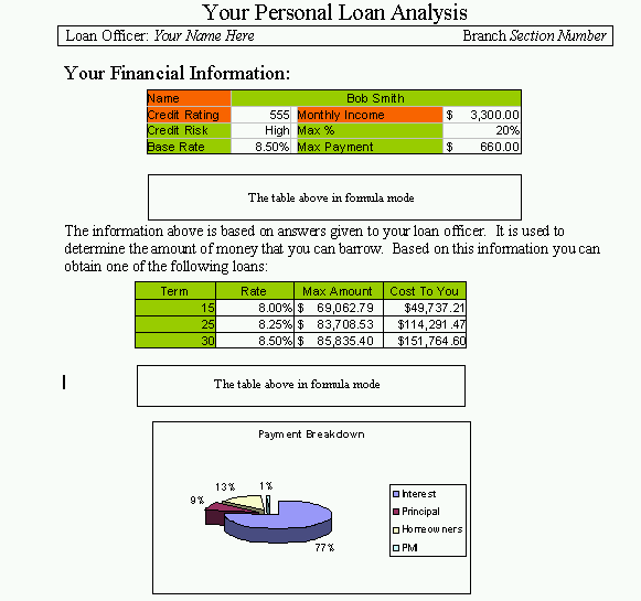
CSCI 104, Spring 2002 Excel Practical

• This project will consist building a personal loan information sheet.
• 
• Please Note: The example document is for Mr Smith, with a credit rating of 555 and a monthly salary of $3,300. You will be need to calculate the information for Ms. Jones, credit rating 875, monthly income $2,800.00.
• Do what you can, save your work often, and turn in what you have completed. Make sure that your name is on the final product.

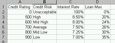
• In Excel, create the flowing chart in cells A1 -> D7. Everything can be input as constants.

  Credit Rating	Risk Class	Interest Rate	Loan Maximum
  0	Unacceptable	100%	0%
  500	High	8.5%	20%
  600	Med. High	8.0%	24%
  700	Average	7.5%	26%
  800	Med. Low	7.25%	30%
  900	Low	7.0%	35%

• 

• In Cell A9, place the label "Name"
• In cells B9-> E9, put the customer's name
• In cell A10, place the label "Credit Rating"
• In Cell B10, place the customer's credit rating
• In cell A11, place the label "Credit Risk"
• In call B11, look up the customer's credit risk automatically
• In cell A12, place the label "Base Rate"
• In cell B12, place the customer's Base interest rate automatically (C2-7)
• In cell D10, place the label "Montly Income"
• In cell E10, place the customer's monthly income
• In cell D11, place the label "Max %"
• In cell E11, place the appropriate value from the Loan Max column of the table above. Look this up automaticaly.
• In cell D12, place the label "Max Payment"
• In cell E12, place the Loan Maximum, this is the percentage from cells (D2-7) multiplied by the customer's monthly income.
• 

• In cell A14, place the label "Term"
• In cell A15, place the value 15
• In cell A16, place the value 25
• In cell A17, place the value 30
• In cell B14, place the label "Rate"
• In cell B15, place the rate B12-0.005
• In cell B16, place the rate B12-0.0025
• In cell B17, place the rate from B12
• In cell C14, place the label "Amount"
• In cell D14, place the label "Cost to you"
• Cells C15-C17, calculate the maximum amount that can be borrowed based on the maximum monthly payment in cell E12, use the goal seek command in each. You will need to use a cell outside of the work area for this computation.
• Cells D15-17 should be the cost of the loan, this is the monthly rate, times the number of payments, minus the amount borrowed.
• 

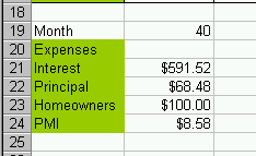
• Label cell A19 "Month"
• Label cell A20 "Expenses"
• Label cell A21 "Interest"
• Label cell A22 "Principal"
• Label cell A23 "Homeowners"
• Label cell A24 "PMI"
• Place in cell B19 40
• Calculate in cell B21, the interest payment for a loan of period specified in A17, for month specified in B19, interest in B17 and principal in C17.
• Calculate in cell B22, the principal payment for a loan of period specified in A17, for month specified in B19, interest in B17 and principal in C17.
• Place in cell B23 100
• Calculate in cell B24, the principal specified in B17 * 0.00001
• Create an exploded pie chart based on the table A20-B24.
• 

• Start word and create the document at the top of the page.
• You should change the customer name to Ms. Jones.
• Change the customer information to
  • credit rating 875
  • monthly income $2,800.00
  • Make sure you recalculate the maximum amounts in cells C15-17
  • Change the month for the chart to 100.
• Place two versions of each table in your document, one in normal mode and one in formula mode.
• Print your document.