Excel Test, Practical Portion.

• Please turn in the written portion of the test if you have not yet done so.
• This portion of the test is open book open notes.
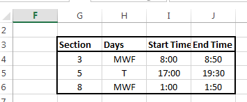
• You must complete this test by the finish time (8:50, 5:50, 1:50)
• Please read the instructions carefully.
• Please compute all values, values typed in will not be given any credit.
  • You may fill in a value by hand if you can not complete a computation and another computation depends upon it.
  • The hand typed value will not receive credit.
• If you fail to email the completed workbook, you will receive no credit.
• Download this file.

1. (1 point) rename sheet1 to Student Information
2. (1 point)
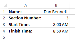
   • Enter your name in cell B1
   • Enter your section number in cell B2
3. (3 points) Format the text in column A,B
   • Adjust the width of columns A and B so that all text fits the cell..
   • Make the titles in column A bold.
   • Format the cells B3 and B4 for time, showing am/pm (you will fill in the data in a few steps)
4. (2 points) Format the data table (G3:J6)
   • Draw a border around the entire table.
   • Draw a border under the headings (G3:j3)
   • Make the headings bold.
   • Center the data in the table.
   • 
5. (5 points) Using the table in G3:J6 look up the start and end time for your test and place these results in cells B3 and B4
   • 
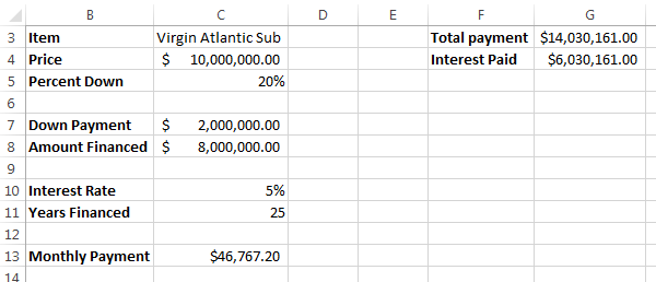
6. Move to the A Loan worksheet. You will calculate information about a loan for a customer purchasing an expensive submarine.
7. (5 points) Simple Computations
   • In cell C7 compute the down payment for this loan based on the price and the percent down.
   • In Cell C8 compute the Amount financed based on the Price and the Down Payment.
8. (5 points) In cell C13, compute the Monthly payment based on the Amount Financed, the Interest Rate and the Years Financed.
9. (2 points) Other Computations
   • In cell G3, compute the total loan amount paid based on the monthly payment and the years financed.
   • In cell G4 compute the interest paid based on the total payment and the amount financed.
   • 
10. Move to worksheet Customer List
    • This worksheet contains a list of customers who are interested in expensive gifts.
      • The customer's name is in column A
      • The gift recipient's age is in column B
      • A code representing the gift the customer wishes to buy is in column C.
    • On the Gift List worksheet is a list of expensive gifts.
      • The Item code is in column B, this matches the code in column C of the previous list
      • A short description is in column C
      • The price of the item is in column D
      • The minimum age to receive this gift is in column E
      • Cell H3 contains the company's discount percentage
      • Cell H4 contains the minimum cost gift to be qualified as a Prime Customer
11. (5 points) Titles
    • Merge the cells and center "Clients Request List" above the table in columns A:J
    • Rotate the column headings by 90degrees (A3:J3)
    • Make the column headings bold, centered, underlined.
    • 
12. (5 points) All computations on this worksheet should be built using appropriate references, so that the formulas can be copied (when appropriate), not retyped.
13. (10 points) Lookups
    • In Column D, lookup the item name based on the Gift Code in column C
    • In column E, look up the item cost based on the Gift code in column C
    • In column H, look up the minimum age based on the Gift code in Column C
    • NOTICE: Do not look up any values by hand, If you are unable to perform these based on a computation, just fill in the first three items and perform the other computations based upon these values.
    • 
14. (5 points) Computations
    • In column F, Compute the discount amount based on the gift cost (col E) and the discount amount (Gift List worksheet cell H3)
    • In column G compute the discount price based on the cost and the discount amount.
15. (10 points) If
    • In column I, place a "Yes" in the cell if the age in column B is greater than the age in column H, otherwise place a "No"
    • In column J, place a "Yes" in the cell if the discount price exceeds the Prime Customer Limit on the Gift List worksheet.
16. Complete the table by copying the formulas to all cells in the table.
17. (5 points) Statistics
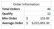
    • In cell M5, compute how many orders were placed based on column A
    • In cell M6, count the number of orders where the customer qualified for the order (based on column I)
    • In cell M7 compute the minimum amount ordered for all orders, based on discount price.
    • In cell M8, compute the average of the orders where the customer qualifies, based on the discount price.
    • 
18. (12 points) Completion/Other Errors
    • Make sure all values are properly formatted and visible.
    • Save the workbook as yourlastname
    • Email a copy of the workbook to