Fall 2009 Excel Test

• If you have not yet done so, please hand in your written portion.
• You may print this document if you wish.
• Please follow all instruction. If you don't understand an instruction, please ask for help.
• You may use your book and notes for this portion of the test.
• Please save frequently.
• All data should be properly labeled and formatted.
• When you finish, make sure that you email a copy of your work to danbennett360@gmail.com.
• All formulas should allow for a change of assumptions.

1. Open chap4_mid1_wedding from your data directory.
   • If you did not bring your usb drive, download this copy of the file
   • Save this file as ExcelTest in your data directory. Make sure that you can find this file later.
2. [2 point] Name
   • Insert a new row above row 1.
   • Place Name in cell A1
   • Place your name in cell B1
   • Make A1 and B1 bold.
3. [8 points] Formatting
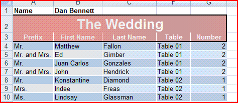
   • Format The Wedding (currently in cell E2) so that it is
     • centered in above the entire table in a single cell
     • 20 point bold
     • text color white
     • background color blue
   • Format the headings in A3:G3
     • bold
     • centered
     • same background color as above
     • same text color as above.
   • Draw a thick border around the headings (A2:G3)
4. [10 points] Data Table
   • Mark A3:G80 as a data table.
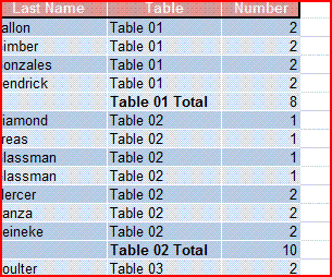
   • Sort the data based on the Table at which the guests are sitting, then by Last Name for each Table.
   • Hide Columns D and E.
   • Add A total line to the bottom of the table, indicating the total number of guests (Column G)
   • 
5. [5 points] Subtotals
   • Find the total number of guests sitting at each table.
   • 
6. [3 points]
   • Save your work so far.
   • Rename the sheet containing the wedding information to Guests
   • Move to sheet2
   • Rename this worksheet Finance
   • Place your name in cell A14
7. [2 points] Enter the following data
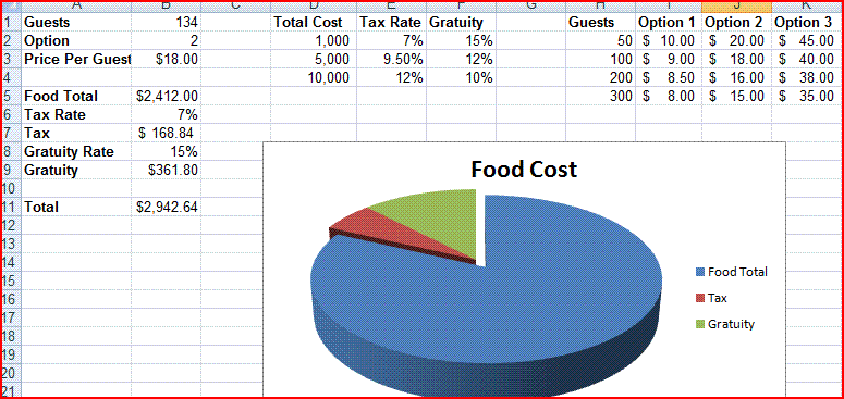
   • In cells D1:K5
   • D1:F4 represent percentage rates based on the Food total.
   • H1:K5 represent the price per guest for three different service choices.
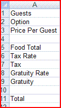
   • In cells A1:A11
   • Make sure that all cells are formatted appropriately and visible.
   • Place 134 in cell B1
   • Place 2 in cell B2.
8. Computations.
   • [3 points] In cell B3 look up the price per guest based on cell B1, B2 and table H1:K5.
     • The initial value should be $18
     • The user should be able to change either B1 or B2 and the computation should be correct.
   • [1 point] Calculate the total cost of the food in cell B5. This should be based on the Guests and the Price Per Guest
   • [2 points] In cell B6, look up the tax rate, based on the Food Total (B5) in table D1:F4
   • [1 point] In cell B7 compute the Tax based on the Food Total (B5) and the Tax Rate (B6).
   • [2 points] In Cell B8 look up the gratuity based on the Food Total (B5) and table D1:F4
   • [1 point] In Cell B9 compute the gratuity based on the Food Total (B5) and the Gratuity Rate (B8)
   • [1 point] In cell B11 compute the total bill based on the Food Total (B5), Tax (B7) and Gratuity (B9)
9. [5 points] Pie Chart
   • Create a pie chart showing a breakdown of the total cost of the meal (B5, B7 and B9)
   • This chart should have the title Food Cost
   • 
10. [4 points]
    • Change to the third worksheet
    • Rename this worksheet to Loan
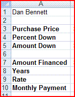
    • Place your name in cell A1
    • In cells A3:A10 place
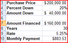
    • Place $200,000 in cell B3
    • Place 30 in cell B8
    • Place 5.25% IN cell B9
11. Financial Computations
    • [5 points] In cell B4 place a formula which will put 20% in the cell if the price (B3) is more than $150,000 and 25% if it is less than or equal to $150,000.
    • [1 point] IN cell B5, compute the Amount Down based on the Purchase Price (B3) and the Percent Down (B4).
    • [1 point] In cell B7 compute the Amount Financed base on the Purchase Price (B3) and the Amount Down(B5)
    • [3 points] In Cell B10 compute the monthly payment based on the Amount Financed (B7), the Years (B8) and the Rate (B9)
    • 
12. Mortgage Table
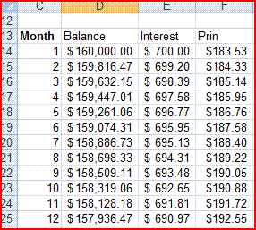
    • In cells C13:F13 enter
    • [1 point] In cells C14:C24 place the numbers 1 through 12
    • [1 point] IN cell D14 place a formula that copies the amount financed from cell B7
    • [4 points] In cell E14 compute the amount of interest for the first month.
      • This is based on the current Balance in cell D14
      • And on the Interest Rate in cell B8 (converted to a monthly interest rate)
      • Make this formula so that it can be copied down to cells E15:E25 so that the interest rate remains the same.
    • [4 points] In cell F14, Compute the amount of the payment that goes to principle
    • Subtract the interest computed in cell E14 from the monthly payment in cell B10
    • You will need to copy this formula down to cells F15:F25 without the monthly payment portion changing.
      • [2 points] In cell D15 compute the new balance due.
        • Subtract the principle (F14) from the Balance (D14)
      • [3 points] Complete the table
        • Copy the formula from D15 to D16:D25
        • Copy the formulas from E14:F14 to E15:F25
      • 

• Do not print the Guests sheet
• Print the Finance and Loan sheets
• Email the final document to danbennett360@gmail.com
• Collect the printouts from the printer and give them to the instructor.
• Penalties for failure to submit
  • Printout : 20 points
  • Email: 75 points