Practical portion, Excel Test

Fall 2006

• Make sure that you save often.
• If you can't do a section, please continue with the next.
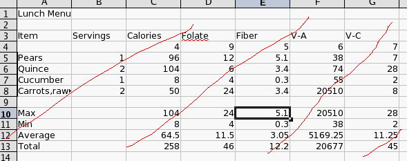
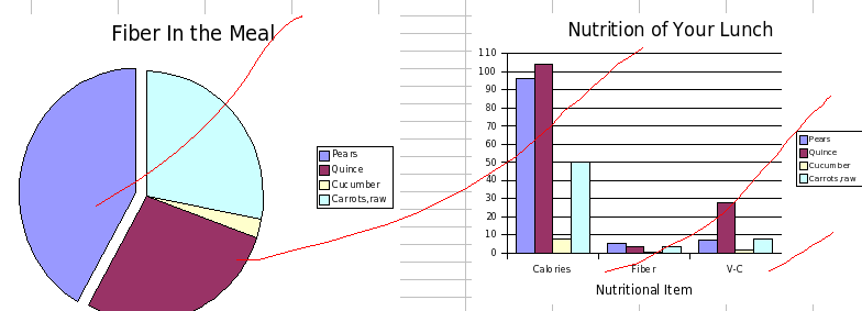
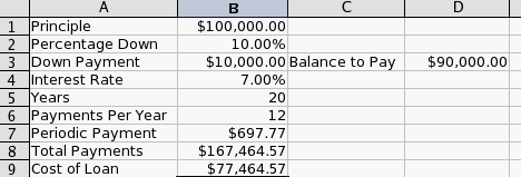
• There are pictures of my document at the end of the instructions. I have added red lines to discourage cheating. Please look at these if you are confused.
• You may print this portion of the test if you wish, but you don't need to.
• When you are finished, you should
  • Mail a copy of the test to dbennett@edinboro.edu

1. Download and save a copy of this file. Please save it to your s drive, then open exel.
2. Part 1, Formatting
   1. All work will be done on the "Nutrition Table" worksheet.
   2. [10 points]
      • Insert a new row at the top of the table
      • Merge all of the cells in this new row
      • Add the title "Nutrition Of Fruits and Vegetables"
      • Center this title
      • Make it 20 point bold.
      • Make the second row so that all the labels fit and can be read.
      • Draw a 4 point line between the second and third row.
      • Freeze the top two rows so that they are always displayed.
      • Set the background of the top two rows to be some light blue color.
      • Place a 2 point border around cells a3 through i154.
      • 
3. Part 2, Formulas and Functions
   1. Go to the "Lunch tab"
   2. We wish to compute the nutritional value of a meal consisting of four different items from the nutrition guide.
   3. Insert the following serving sizes in column B : 1 2 1 2
   4. [1 point] Between Rows 3 and 4 insert a new row.
   5. [1 point] In this row, add the number of the column in which each item is located. (So C5 should contain a 9, as this is the column in the Nutrition table that holds Folate). Type these numbers into the cells.
   6. [5 points]
      • Using the data in row 4, develop a formula that will compute the nutritional information for the items in column A, with servings listed in column B.
      • You should be able to copy this formula to all the other cells in the table.
      • Complete this table.
   7. [3 points] Find the maximum, minimum, average, and total for all columns in the table.
   8. Row 15 contains the USRDA values for each item. For calories it is a minimum, for everything else it is a maximum.
      • [5 points] In row 16, place the word Over if the total for that item is over the USDA, and Under if the total for that item is under the USDA.
      
   9. [5 points] Produce a pie chart showing the Fiber contribution of each item in the table.
   10. [5 points] Produce a column chart showing the the contribution of each item for Calories, Folate and Vitimin C.
4. Part 3, Financial Functions.
   1. [2 points] Insert a new worksheet entitled Financial Functions
   2. [2 points] Build the basic table:
      • In cell A1 Enter Principle
      • In cell B1 Enter 100,000
      • In cell A2 Enter Percentage Down
      • In cell B2 Enter 10%
      • In cell A3 Enter Down Payment
      • In cell C3 Enter Balance to Pay
      • In cell A4 Enter Interest Rate
      • In cell B4 Enter 7%
      • In cell A5 Enter Years
      • In cell B5 Enter 20
      • In cell A6 Enter Payments Per Year
      • In cell B6 Enter 12
      • In cell A7 Enter Periodic Payment
      • In cell A8 Enter Total Payments
      • In cell A9 Enter Cost of Loan
   3. [1 point] Compute the down payment in cell B3 by multiplying the principle by the percentage down.
   4. [1 point] Compute the balance to pay in D3 by subtracting the down payment from the principle
   5. [4 points] Compute the periodic payment in cell B7 based on the balance to pay, interest rate, years, and payment per year.
   6. [1 point] Compute the total of all payments in B8 by multiplying the periodic payment by the total number of payments.
   7. [1 point] Compute the cost of the loan by subtracting the balance to pay from the total payments.
   8. [3 points] Change the values as follows

      Cell	New value
      B1	60,000
      B2	3%
      B5	30
      B6	26