Excel Test, Fall 2002

For this test you will produce a power point presentation. You will need to use excel to produce most of the slides.

When you are finished, please print out the slide show 6 slides per page.

Title Slide
- Title: Test 2
- Sub Title:
  - Your Name
  - The start time of your class
  - Fall 2002
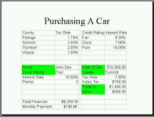
First Slide: Purchasing A Car
- Insert the spread sheet described below in normal mode,
- Cell B9 should contain Poor
- Cell B11 should contain 5
- Cell E8 should contain 10,000
- Cell E9 should contain Summit
- Cell E12 should contain 1,000
- Cell E13 should contain 400
Second Slide: Purchasing A Car
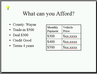
Third Slide: What Can you Afford
- Use the Goal Seek Command to find how much car a person can afford if
  - They live in Wayne County
  - They have a trade in worth $500
  - They have a $300 other value
  - The have a good credit rating
  - They want to finance the car for 4 years.
- Find The vehicle pirice for a monthly payment of
  - $300
  - $400
  - $500
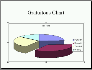
Last Slide: Gratuitous Chart
- Make An exploded pie chart out of the table in A1 through B5
- Explode out the entry for Summit County only.

The spreadsheet

In Column A and B, Rows 1 through 5 enter the following table:

County Tax Rate

Portage 1.75%

Summit 2.50%

Trumbull 2.00%

Wayne 1.00%

Portage 1.75%
In Column D and E, rows 1 through 4 enter the following table:

Credit Rating Interest Rate

Fair 8.50%

Good 7.00%

Poor 10.00%
In A8 put the constant "Name", color this cell green
In A9 put the constant "Credit Rating", color this cell green as well
In A10 put "Interest Rate"
In A11 put "Period"
Enter a your name in B8
Enter "Good" in B9
use vlookup and the chart D1:E4 along with B9 to fill in the interest rate in B10
Put a 5 in B11
Put "Cost of Car" in D8, color this cell green
Put "County" in D9, color this cell green
Put "Tax Rate" in D10
Put "Sales Tax" in D11
Put "Trade In" in D12, color this cell green.
Put "Other" in D13, color this cell green.
Put 10,000 in E8
Put "Summit" in E9
Use Vlookup on the table A1:B5 and the county in E9 to find the tax rate in cell E10, Add 6% to the value looked up in the table.
Calculate the sales tax: Price of Car times Tax Rate in E11
Put 1,000 in E12
Put 400 in E13
Put "Total Financed" in A15
Put "Monthly Payment" in A16
Calculate the total Financed in B15 (Cost + sales tax - trade in - other)
Calculate the monthly payment in B16

Note, when finding values for the slide show, only change the cells associated with labels in green. My Slides look something like: