Adjusting Worksheet Views

• Freezing and unfreezing panes
  • As worksheets become larger it is important to keep the labels visible as you move throughout the worksheet.
  • Freezing rows and columns are very useful
• Splitting screens horizontally and vertically
  • This will allow you to see multiple (disjoint) portions of a worksheet at the same time.
  • Again, this is useful with large worksheets.
• Showing necessary information with the outlining feature
  • This seems a nice feature.
  • Especially if you are presenting in a meeting or conference.

A house loan

• Start a new workbook
• In this workbook, we will model a house purchase.
• The house we will purchase costs $120,000, the bank requires 20% down and has an interest rate of 3.754% for 30 years.
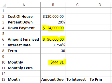
• Set up the first part of the worksheet as follows
  • 
  • The items in yellow should be computations
    • B4 is the price of the house times the percent down
    • B6 is the price of the house minus the down payment
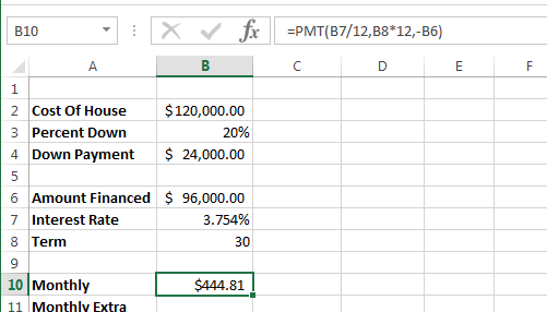
    • B10 uses the payment function
      • =pmt(interest rate per payment, number of payments, amount)
      • In this case, the interest rate will be cell B7/12
      • The number of payments will be B8*12
      • The amount will be -B6
      • 
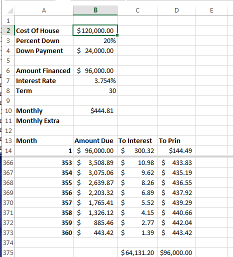
• Next we will set up an amortization table.
  • Put the numbers 1 through 360 (ie 12 * 30) in A14:A373
  • In cell B14 just copy the amount financed
  • In cell C14 copy the interest due for the first month
    • This is a simple interest loan for one month
    • It should be the amount due (B14)
    • Multiplied by the monthly interest rate (B7/12)
    • 
  • In Cell D14 compute the amount that goes to pay off the loan
    • This is the monthly payment (B10) minus the interest in cell C14
  • In cell B15 calculate the new amount due (for month 2)
    • This is the old amount due (B14)
    • Minus the amount to principle (D14)
    • Minus any extra payment we want to make each month (B11)
  • Formulas:
  • 
  • Data values:
  • 
  • Copy these values down to fill in the rest of the table.
  • Finally in Cells C375 and D375, calculate the sum of each of these columns (C14:C373), (D14:D373)
  • 
• Click in cell B14 and select Freeze Panes, Freeze Panes on the VIEW tab.
• Scroll around and see what happens
• Click on column 15 and click on Split int he VIEW tab.
  • 
  • You should now have two screens.
  • Click in the bottom and scroll down to month 360
  • Notice that the last payment matches the last amount due.
  • And the sum of To Prin matches the Amount Financed
• Adjust some values in cells B2:B13
  • Change the interest rate to 6%
  • Change the cost of the house to $350,000
  • Put $1 in cell B11