Data Analysis Tools

• Using Goal Seek
  • Goal seek is really cool.
  • And very easy to use.
  • But the use is limited a single variable.
  • Watch this one of no others in this series.
• Using Solver
  • This is a more powerful version of goal seek.
  • But it is more complex as well.
  • This is probably worth a watch just to see what is happening.
• Using Scenario manager
  • This allows you to set up a spreadsheet where you can quickly change multiple different values.
• Using data tables.
  • A really cool way to copy a formula across an entire table.
• If you are really enjoying this, look at chapter 15, Macros
• If you like that, come and talk to me.

Do I make the grade?

• Start with this worksheet
• You may feel free to change the scores, I have used estimates.
• Setup
  • Compute the points in column D, score in column C * percent of grade in column B
  • Compute the total of the points in D10
  • in D11, do a vlookup of the total points in the grade table.
• Goal Seek
  • We will investigate what it will take to get an A with these grades.
  • We cod do this by trial and error, but why not let excel do this for us.
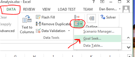
  • Select Goal Seek (Data tab, Data Tools, What If Analysis, Goal Seek)
  • 
  • Select cell d10 as the Set Cell value.
  • It looks like this person can't get an "A",
  • What do they need to get a "B"
• Solver
  • Goal seek limits us to changing one value
  • Solver lets us change many.
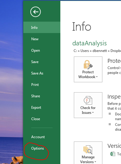
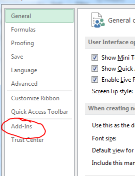
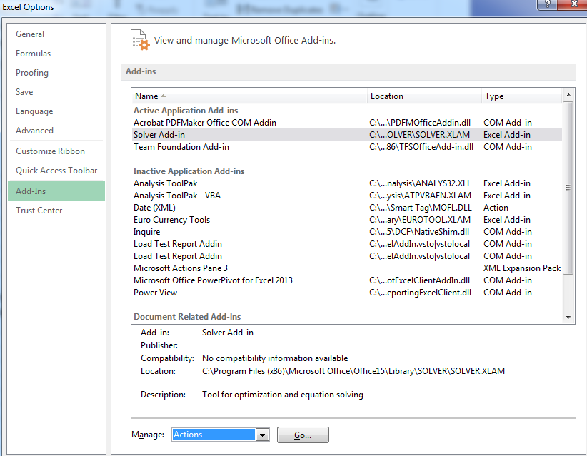
  • FILE, Options, Ad-Ins, Select Solver, ok.
  • 
  • 
  • Note, Mine is already active, you may have to activate yours.
  • 
  • Start Solver: Data: Solver
  • 
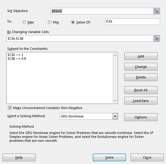
  • Set Objective: D10
  • To value of: 90
  • By changing variable cells: C4, C8
  • Add the rule C4 <=1 and C8 <= .9
  • 
• Data Tables
  • Rather different sort of thing.
  • I would like to construct a table that demonstrates the power of compound interest.
  • This will use the formula A = P(1+r/n)^(nt)
    • A is the final amount, what we want to compute
    • P is the principle
    • r is the annual interest rate
    • t is the number of years we will invest the money
  • Move to the compound Interest worksheet
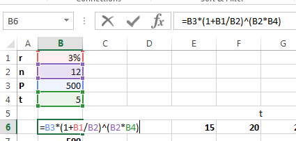
  • In cell b6 enter the formula
  • 
  • Format it as money.
  • Highlight B6:j26
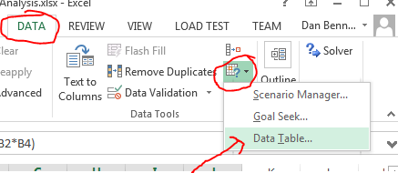
  • On the Data tab select What if Analysis, Data Table
  • 
    • The row input cell is b4
    • The column input cell is b3
  • Notice, you can change all values (b1, B2, C6:j6, b7:b26) and the table will change.
• Scenario Manager
  • Return to the Grade Computation worksheet.
  • We will now set up some scenarios
    • You would like to present some possible outcomes for the class.
    • Different results for study and work for example.
  • Go to Data, What-If analysis, and select Scenario Manager
  • Start by adding a default scenario
    • Click Add
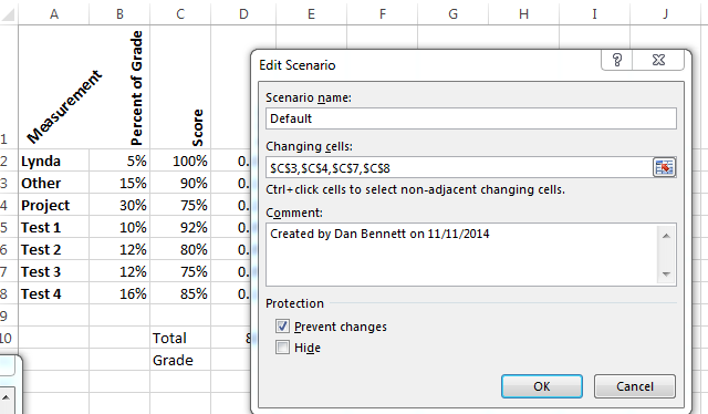
    • Name the scenario Default
    • Select the scores you can yet change (C3, C4, C7, C8)
    • 
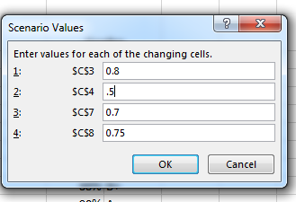
    • Add another scenario for low grades
    • Call it low grades
    • .8, .5, .7 and .75
    • 
    • Click on show to show this scenario